This week end I worked with the DrawIndexedInstancedIndirect function, and since I didn’t find that much informations I wanted to share my results.

The next step for my voxel cone tracing project was to generate mip maps for my voxel grid. I implemented a first draft, but I needed a better way of displaying my voxel grid, to make sure that they all of them were correct.

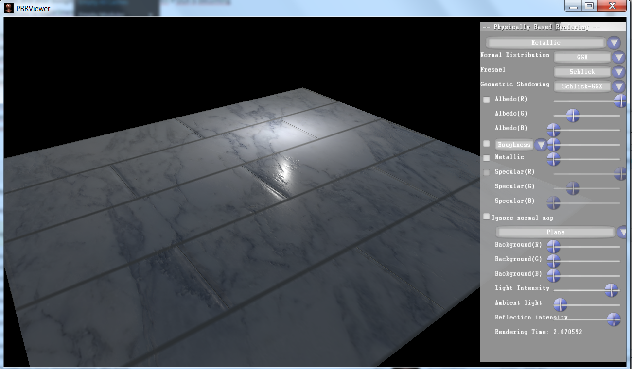
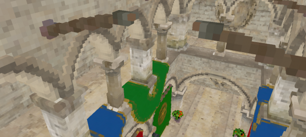
I was using the depth map to compute the world position. Then I transformed it into voxel grid coordinates to find the color of the matching voxel.

The problem is that, as shown in the screenshot, it doesn’t allow seeing the real voxelized geometry, and it’s hard to have a clear idea of the imprecision induced by the voxels.

That’s why I started to work on a way to draw all voxels, using the DrawIndexedInstancedIndirect function. Draw instanced allows to draw several times a unique object, here I just draw a simple cube, and to apply instance specific parameters on each of them.

The “indirect” functions are the same as the “non indirect” ones, except that the arguments are contained in a buffer. It means that the CPU doesn’t have to be aware of the arguments of the function, it can be created by a compute shader, and directly used to call another function.

I have a buffer containing all my voxels, and the first thing I wantto know  is how many of them are not empty (that will be the number of instances to draw), and their positions within my voxel grid.

The first step is to create the buffer that will be used to feed the DrawIndexedInstancedIndirect function:

D3D11_BUFFER_DESC bufferDesc;

ZeroMemory(&bufferDesc, sizeof(bufferDesc));
bufferDesc.ByteWidth = sizeof(UINT) * 5;
bufferDesc.Usage = D3D11_USAGE_DEFAULT;
bufferDesc.BindFlags = D3D11_BIND_UNORDERED_ACCESS;
bufferDesc.CPUAccessFlags = 0;
bufferDesc.MiscFlags = D3D11_RESOURCE_MISC_DRAWINDIRECT_ARGS;
bufferDesc.StructureByteStride = sizeof(float);

hr = m_pd3dDevice->CreateBuffer(&bufferDesc, NULL, pBuffer);

The important flag here is D3D11_RESOURCE_MISC_DRAWINDIRECT_ARGS, to specify that the buffer will be used as a parameter for a draw indirect call.

Next, the associated unordered access view to be able to write into it from a compute shader.

D3D11_UNORDERED_ACCESS_VIEW_DESC uavDesc;
ZeroMemory(&uavDesc, sizeof(uavDesc));
uavDesc.Format = DXGI_FORMAT_R32_UINT;
uavDesc.ViewDimension = D3D11_UAV_DIMENSION_BUFFER;
uavDesc.Buffer.FirstElement = 0;
uavDesc.Buffer.Flags = 0;
uavDesc.Buffer.NumElements = 5;

hr = m_pd3dDevice->CreateUnorderedAccessView(*pBuffer, &uavDesc, pBufferUAV);

As I said early I need to be able to know the position of the voxels in the voxel grid, to be able to find their position in the world, and I’ll be able to find their color. For that I use an Append Buffer,  an other usefull type of buffer that behave pretty much like a stack. When you “Append” a data, it will be put at the end of the buffer, and an hidden counter of element will be incremented.

Here is how I created this buffer and the associated SRV and UAV:

void Engine::CreateAppendBuffer(ID3D11Buffer** pBuffer, ID3D11UnorderedAccessView** pBufferUAV, ID3D11ShaderResourceView** pBufferSRV, const UINT pElementCount, const UINT pElementSize)
{
    HRESULT hr;

    D3D11_BUFFER_DESC bufferDesc;
    ZeroMemory(&bufferDesc, sizeof(bufferDesc));
    unsigned int stride = pElementSize;
    bufferDesc.ByteWidth = stride * pElementCount;
    bufferDesc.Usage = D3D11_USAGE_DEFAULT;
    bufferDesc.BindFlags = D3D11_BIND_SHADER_RESOURCE | D3D11_BIND_UNORDERED_ACCESS;
    bufferDesc.CPUAccessFlags = 0;
    bufferDesc.MiscFlags = D3D11_RESOURCE_MISC_BUFFER_STRUCTURED;
    bufferDesc.StructureByteStride = stride;

    hr = m_pd3dDevice->CreateBuffer(&bufferDesc, NULL, pBuffer);

    if(FAILED(hr))
    {
        MessageBox(NULL, L"Error creating the append buffer.", L"Ok", MB_OK);
        return;
    }

    D3D11_UNORDERED_ACCESS_VIEW_DESC uavDesc;
    ZeroMemory(&uavDesc, sizeof(uavDesc));
    uavDesc.Format = DXGI_FORMAT_UNKNOWN;
    uavDesc.ViewDimension = D3D11_UAV_DIMENSION_BUFFER;
    uavDesc.Buffer.FirstElement = 0;
    uavDesc.Buffer.Flags = D3D11_BUFFER_UAV_FLAG_APPEND;
    uavDesc.Buffer.NumElements = pElementCount;

    hr = m_pd3dDevice->CreateUnorderedAccessView(*pBuffer, &uavDesc, pBufferUAV);

    if(FAILED(hr))
    {
        MessageBox(NULL, L"Error creating the append buffer unordered access view.", L"Ok", MB_OK);
        return;
    }

    D3D11_SHADER_RESOURCE_VIEW_DESC srvDesc;
    ZeroMemory(&srvDesc, sizeof(srvDesc));
    srvDesc.Format = DXGI_FORMAT_UNKNOWN;
    srvDesc.ViewDimension = D3D11_SRV_DIMENSION_BUFFER;
    srvDesc.Buffer.FirstElement = 0;
    srvDesc.Buffer.NumElements = pElementCount;

    hr = m_pd3dDevice->CreateShaderResourceView(*pBuffer, &srvDesc, pBufferSRV);

    if(FAILED(hr))
    {
        MessageBox(NULL, L"Error creating the append buffer shader resource view.", L"Ok", MB_OK);
        return;
    }
}

Now, the compute shader. It’s in fact pretty simple. First step, the first thread initialize my argument buffer to 0, except for the first argument that represent the number on indices in the index buffer that will be bind.

Then, each time I found a non empty voxel, I increase the number of instances to draw using an InterlockedAdd, and I append it’s position in the perInstancePosition buffer.

AppendStructuredBuffer < uint3 > perInstancePosition:register(u0);

RWStructuredBuffer < Voxel > voxelGrid:register(u1);

[numthreads(VOXEL_CLEAN_THREADS, VOXEL_CLEAN_THREADS, VOXEL_CLEAN_THREADS)]
void main( uint3 DTid : SV_DispatchThreadID )
{
    if ( DTid.x + DTid.y + DTid.z == 0)
    {
        testBuffer[0] = 36;
        testBuffer[1] = 0;
        testBuffer[2] = 0;
        testBuffer[3] = 0;
        testBuffer[4] = 0;
    }
    GroupMemoryBarrier();

    uint3 voxelPos = DTid.xyz;
    int gridIndex = GetGridIndex(voxelPos);

    if (voxelGrid[gridIndex].m_Occlusion == 1)
    {
        uint drawIndex;
        InterlockedAdd(testBuffer[1], 1, drawIndex);

        VoxelParameters param;
        param.m_Position = voxelPos;
        perInstancePosition.Append(param);
    }
}

At the end of the execution of this computer shader the buffers are both filled with the information needed to draw all the voxels.

I use a really simple cube to represent the geometry of a voxel:

// Create the voxel vertices.
VertexPosition tempVertices[] =
{
    { XMFLOAT3( -0.5f,  0.5f, -0.5f )},
    { XMFLOAT3(  0.5f,  0.5f, -0.5f )},
    { XMFLOAT3(  0.5f,  0.5f,  0.5f )},
    { XMFLOAT3( -0.5f,  0.5f,  0.5f )},

    { XMFLOAT3( -0.5f, -0.5f, -0.5f )},
    { XMFLOAT3(  0.5f, -0.5f, -0.5f )},
    { XMFLOAT3(  0.5f, -0.5f,  0.5f )},
    { XMFLOAT3( -0.5f, -0.5f,  0.5f )},
};

// Create index buffer
WORD indicesTemp[] =
{
    3,1,0,
    2,1,3,

    6,4,5,
    7,4,6,

    3,4,7,
    0,4,3,

    1,6,5,
    2,6,1,

    0,5,4,
    1,5,0,

    2,7,6,
    3,7,2
};

I can now bind this index and vertex buffer, the perInstancePosition and voxelGrid buffers, and start to write the shaders. The goal is simple, each item in the perInstancePosition is a uint3 reprensenting the position of a “non empty” voxel in the voxel grid. I just need to move the vertices to the right world position, increase the size of my unit cube to match the size of a voxel, and to find the right color to pass it to the pixel shader.

Here is my vertex shader:

#include "VoxelizerShaderCommon.hlsl"

StructuredBuffer < uint3 > voxelParameters: register(t0);
StructuredBuffer < Voxel > voxelGrid: register(t1);

cbuffer ConstantBuffer: register(b0)
{
    matrix g_ViewMatrix;
    matrix g_ProjMatrix;
    float4 g_SnappedGridPosition;
    float g_CellSize;
}

struct VoxelInput
{
    float3 Position : POSITION0;
    uint InstanceId : SV_InstanceID;
};

struct VertexOutput
{
    float4 Position: SV_POSITION;
    float3 Color: COLOR0;
};

VertexOutput main( VoxelInput input)
{
    VertexOutput output;

    uint3 voxelGridPos = voxelParameters[input.InstanceId];

    int halfCells = NBCELLS/2;

    float3 voxelPosFloat = voxelGridPos;

    float3 offset = voxelGridPos - float3(halfCells, halfCells, halfCells);
    offset *= g_CellSize;
    offset += g_SnappedGridPosition.xyz;

    float4 voxelWorldPos = float4(input.Position*g_CellSize + offset, 1.0f);

    float4 viewPosition = mul(voxelWorldPos, g_ViewMatrix);
    output.Position = mul(viewPosition, g_ProjMatrix);

    uint index = GetGridIndex(voxelGridPos);
    output.Color = voxelGrid[index].Color;

    return output;
}

An interesting thing here is the instanceId, automatically created by the draw instanced command, that  identify each instance, allowing me to create a voxel for each position in the buffer.

The pixel shader is really straightforward:

struct VertexOutput
{
    float4 Position: SV_POSITION;
    float3 Color: COLOR0;
};

float4 main(VertexOutput input) : SV_TARGET
{
    return float4(input.Color, 1.0f);
}

And finally I call the DrawIndexedInstancedIndirect function :

engine->GetImmediateContext()->DrawIndexedInstancedIndirect(argBuffer, 0);

This is just an example, but the draw indirect functions allow to do a lot of things using only the gpu, without the need to synchronise with the cpu. It’s a powerfull tool, and I really want to try more stuff whith that.

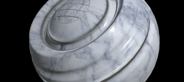
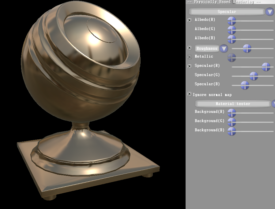
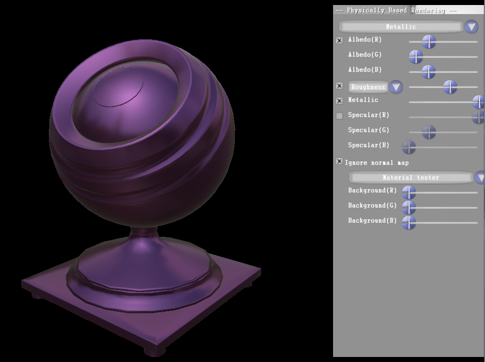
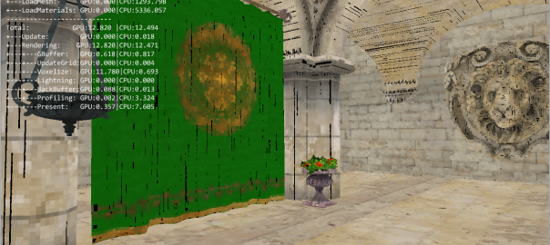
And to conclude, some screenshots for voxels grid of 32x32x32 and 256x256x256: